As an example of the multiple regression analysis discussed in the previous post, let's look at how to predict home prices using the California housing dataset. We'll walk through the process of loading the data, splitting it into training and test sets, creating a linear regression model, training the model, making predictions, and evaluating the model's performance.

Dataset:

The California housing dataset contains data on various factors that potentially influence housing prices, such as the median income, housing median age, average number of rooms, and average number of occupants per household. The dataset consists of 20,640 samples and 8 independent variables.

Loading the Data:

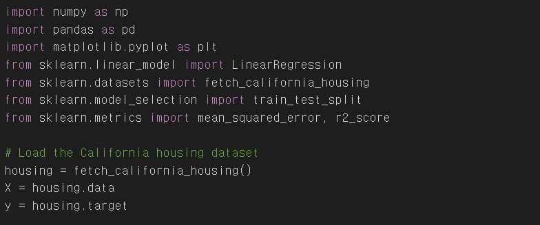
First, we import the necessary libraries and load the California housing dataset using the 'fetch_california_housing()' function from the 'sklearn.datasets' module.

Splitting the Data: 

We split the dataset into training and testing sets using the 'train_test_split()' function from the 'sklearn.model_selection' module. The 'test_size' parameter (0.2) indicates that 20% of the data will be reserved for testing, and the remaining 80% will be used for training. The 'random_state' parameter (42) ensures that the data is split consistently across multiple runs, allowing for reproducible results.

Creating and Training the Model:

Next, we create a linear regression model using the 'LinearRegression()' class from the 'sklearn.linear_model' module. Then, we train the model on the training data using the 'fit()' method, which adjusts the model's parameters to minimize the error between the predicted and actual values.

Making Predictions:

We use the trained model to predict housing prices for the testing data using the 'predict()' method. This generates an array of predicted prices ('y_pred') corresponding to the input features in the testing dataset ('X_test').

Evaluating Model Performance:

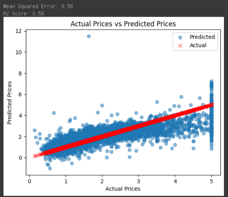
We evaluate the model's performance by calculating the mean squared error (MSE) and R2 score using the 'mean_squared_error()' and 'r2_score()' functions from the 'sklearn.metrics' module. The MSE measures the average squared difference between the predicted and actual values, while the R2 score represents the proportion of variance in the dependent variable that is predictable from the independent variables

Visualizing the Results:

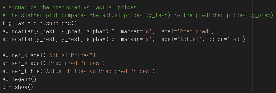
Finally, we visualize the predicted vs. actual prices using a scatter plot from the 'matplotlib.pyplot' library. The 'alpha' parameter (0.5) controls the transparency of the points, making it easier to see overlapping data points. This code modifies the previous scatter plot to display predicted prices as circles (marker='o') and actual prices as crosses (marker='x'). The red color is used for the actual prices to make them stand out. The legend is added to help distinguish between the actual and predicted values.

 

In this example, we demonstrated how to apply Multiple Linear Regression to predict housing prices using the California housing dataset. We went through the steps of loading the data, splitting it into training and testing sets, creating a linear regression model, training the model, making predictions, and evaluating the model's performance.

By calculating the mean squared error and R2 score, we were able to assess the model's performance quantitatively. The scatter plot allowed us to visualize the relationship between the actual and predicted housing prices, giving us a sense of how well the model is performing.

It is essential to note that this example serves as an introduction to the application of Multiple Linear Regression. In practice, further steps such as feature scaling, feature selection, and hyperparameter tuning may be necessary to improve the model's performance. Additionally, other regression techniques or machine learning algorithms might be more suitable for specific datasets or problem domains.