Probability distributions are widely used in data analysis to model various phenomena, understand data patterns, and make informed decisions.  

1. Predict data trends and patterns: 

Probability distributions can help describe your data by providing insights into the central tendency (mean, median, mode), dispersion (variance, standard deviation), and shape (skewness, kurtosis) of your data, allowing you to better understand your data and identify potential trends or patterns.  

2. Hypothesis testing and confidence intervals: 

Hypothesis testing is used to compare your sample data to the null hypothesis and determine the statistical significance of your results. It also helps you construct confidence intervals that provide a range of values for a population parameter based on your sample data.

3. Regression analysis: 

Regression analysis uses probability distributions to estimate relationships between variables and predict outcomes. For example, linear regression analysis assumes a normal distribution for the error term.

4. Time series analysis and forecasting: 

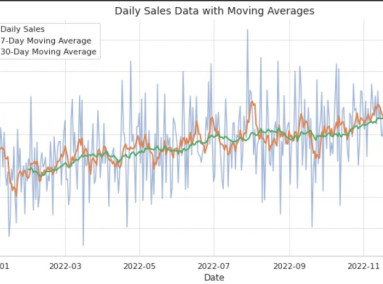
In time series analysis, probability distributions can be used to model trends, seasonality, and noise components in data. This allows businesses to predict the future value of key metrics, such as sales or demand, and make informed decisions about resource allocation, pricing, or inventory management.

Probability distributions are mathematical representations of the likelihood of various outcomes in statistical experiments like these. Understanding the different types of probability distributions and their strengths and weaknesses can help you choose the right model for your data and make more informed decisions.

Let's take a look at the main types of probability distributions and discuss the advantages and disadvantages of each.

1. Discrete probability distributions

Discrete probability distributions are used when the possible outcomes are finite or countable. 

1) Discrete uniform distribution

A discrete uniform distribution assigns equal probability to all possible outcomes and is often used when there is no prior information or knowledge about the likelihood of different outcomes. Examples include throwing a die.

- Pros: Simple and easy to understand, and can be performed with minimal information about the data. No need to estimate parameters.

- Cons: Assumes equal likelihood, which may not be realistic in many scenarios.

2) Bernoulli distribution 

The Bernoulli distribution models a single binary outcome, such as success or failure. It is typically expressed as 'p' for the probability of success and '1-p' for the probability of failure. Examples include flipping a coin (assuming heads as success and tails as failure).

- Pros: Great for independent events or tests, and are characterized as simple and easy to understand. 

- Cons: Assumes a constant probability of success, and is limited to binary outcomes (success or failure).

3) Binomial distribution

The binomial distribution is an extension of the Bernoulli distribution and models the number of successes in a fixed number of independent Bernoulli trials, each with the same probability of success (p).

- Pros: Can be used to model a variety of real-world scenarios, and can model the distribution of binomial outcomes across multiple trials.

- Cons: Assumes a constant probability of success across multiple trials, and like the Bernoulli distribution, is limited to binary outcomes (success or failure).

4) Poisson distribution

The Poisson distribution models the number of events that occur in a fixed interval of time or space as a constant average rate.

- Pros: Allows you to model infrequent events over a specified interval.

- Cons: Assumes a constant mean rate and independence of events, and may not be suitable for modeling non-stationary processes.

2. Continuous probability distribution

Continuous probability distributions are used when the possible outcomes are uncountable or infinite. 

1) Continuous uniform distribution

A continuous uniform distribution assigns equal probability to all possible outcomes within a specified range. It is often used when there is no preference or knowledge of the likelihood of different outcomes within the range.

- Pros: Simple and easy to understand, and can be done with minimal information about the data.

- Cons: Very limited in application as it assumes equal likelihood, which may not be realistic in many scenarios.

- Characteristics: It has the same probability density for each outcome within a given interval (a, b). 

Shape of the graph: Has a rectangular shape with constant height inside the interval (a, b) and zero height outside the interval.

Example: A random number is selected between 0 and 1, and all numbers within this interval have the same probability of being selected.

2) Normal distribution (Gaussian distribution)

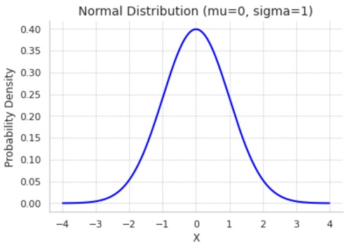
The normal distribution, also known as the Gaussian distribution, has a bell-shaped graph characterized by a mean (μ) and standard deviation (σ). 

The central limit theorem (CLT) states that the sum or mean of a number of independent and identically distributed random variables, regardless of their individual distributions, converges to a normal distribution as the number of variables increases. Because of this powerful result, the normal distribution can be applied to a wide variety of real-world problems and statistical procedures, making it one of the most widely used probability distributions.

However, it requires that the random variables be independent and identically distributed, and that the variables have a finite mean and variance.

- Pros: Applicable in a wide range of situations, and can be used to model many real-world phenomena through the central limit theorem.

- Cons: Assumes symmetry, so may not be suitable for all data, may not be suitable for modeling extreme events or heavy-tailed distributions.

- Characteristics

1. defined by two parameters: mean (μ) and standard deviation (σ).

2. the probability density function (PDF) is defined as (1 / (σ * √(2 * π))) * exp(-(x - μ)² / (2 * σ²)))

3. the shape of the graph: The normal distribution has a symmetrical bell shape with the highest probability density at the mean (μ) and decreasing density as you move away from the mean. The tail of the distribution asymptotically approaches the x-axis but never touches it.

I realize that the above characteristics may be a bit overwhelming for the uninitiated, so skip ahead for now. We'll just need to understand what data we need to apply this normal distribution to later, implement it in Python code, and put it to work!

The normal distribution assumes symmetry, but other probability distributions, such as the lognormal or gamma distribution, may be more appropriate for real-world data that is not symmetric or exhibits other characteristics. However, covering all of these different probability distributions would be overwhelming. 

We recommend that you first try out some of the more common probability distributions in your work to familiarize yourself with the characteristics of your data and the properties of probability distributions, and then dive into the different probability distributions!

In the next post, we'll implement them in Python code with examples so that you can use them in your work.