I was prompted to write a continuation of my previous post due to exceeding the character length I could write in a post. 

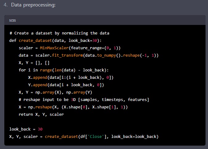
4. This is the data preprocessing part, which involves processing the dataset into a form that can be input to the LSTM model.

The create_dataset() function processes the input data (data) into a dataset for prediction using data over a period of time (look_back). The input data is normalized to values between 0 and 1 using MinMaxScaler() and transformed into a 2D tensor using the reshape() function. We then create the dataset by traveling the length of the look_back to generate the input and output data.

We generate the input data (X) and output data (Y) through a loop and convert them to numpy arrays. Finally, we convert and return them in the form of 3D tensors that the LSTM model can use. The scaler variable is a MinMaxScaler object used to convert the normalized values back to real prices.

The look_back variable defines the time step of the data to be input to the LSTM model (the number of previous data points in the time series data to use as input). This value is used to scale the input to the model.

Finally, the transformed dataset and the scaler object are stored in the X, Y, and scaler variables. X is the 3D tensor that will be input to the model, and Y is the outcome that the model will predict (the actual outcome). The scaler object will later be used to convert the predicted outcome from scaled values back to actual prices.

5. This is the part where you create the Long Short-Term Memory (LSTM) model.

First, a sequential model is created using the Sequential() function, and LSTM layers are added in turn using the model.add() function.

The first LSTM layer has 64 neurons, and we set return_sequences=True to pass the output of the LSTM to the next layer. 

The input_shape argument is where we define the size of the input data.

 The input_shape=(1, look_back) defines the dimensions of the 3D tensor (batch_size, time_steps, input_dim) except for the first dimension (batch_size), which is defined as (1, look_back).

The second LSTM layer has 32 neurons, and we set return_sequences=False so that the output is not passed to the next layer.

The last layer is created using the Dense() function, which has one output neuron and is set to Dense(1) because it is the final predicted value.

To compile the model, we use the compile() function. The loss argument specifies the loss function, which we set to mean_squared_error. We used ADAM as the optimization algorithm.

7. Separating train/test Data:

The reason for separating train and test data in deep learning is to evaluate the generalization performance of the model, i.e., to ensure that the model is not overfitted to the train data and generalizes well to new data.

Train data is the data used to train the model, and test data is the data used to evaluate the model's generalization performance. 

Since deep learning models are optimized for train data, it is important to make sure that the model is not overfitted to the train data and performs well on the test data as well.

With an 80:20 split, you use 80% of the total dataset as train data and 20% as test data. This method is very simple and effective. The advantages of an 80:20 split include

1) Efficient model training: As the size of the train data increases, the model is trained more effectively. Using 80% of the data as train data ensures that the model is trained with enough data.

2) Effective generalization performance evaluation: The smaller the size of the test data, the more effective it is for evaluating the generalization performance of the model. Using 20% of the data as test data allows the model to evaluate its generalization performance well.

8. Generate and plot the predicted prices

The code below is the part that uses the trained model to generate predicted price data and visualizes the prediction results for the training and test datasets.

The model.predict() function was used to generate the prediction results for the training and test datasets, and the generated prediction results are stored in the train_predict and test_predict variables.

Since the results predicted by the model represent normalized values, we used the scaler.inverse_transform() function to rescale them and convert them to actual price values. 

This function is used to convert the scaled values of the training dataset (train_Y) and test dataset (test_Y) back to real prices. 

The results of this transformation are stored in the variables train_predict, train_Y, test_predict, and test_Y.

Finally, we use the matplotlib library to visualize the training dataset, test dataset, and prediction results. 

Use the plt.plot() function to plot a line graph for each dataset; use the plt.legend() function to add a legend; use the plt.title(), plt.xlabel(), and plt.ylabel() functions to specify the title, x-axis label, and y-axis label of the graph, respectively; and use the plt.show() function to output the graph to the screen.

9. Deep Learning Training Screen

10. Cryptocurrency price forecasts predicted by LSTM models 

In addition to these price forecasts, data analysts can contribute to the organization by performing causal analysis and future predictions from historical data. 

1) Data-driven decision-making: Organizations can formulate and execute data-driven strategies, which helps in making the organization more competitive.

2) Improving efficient processes: By analyzing processes and systems, you can find out where improvements can be made, solve problems, and reduce costs.

3) Improve business performance: By analyzing data within your organization, you can determine strategies that can improve business performance to increase revenue, reduce costs, and increase customer satisfaction.

4) Gain a competitive advantage: It helps organizations stay competitive. They help organizations discover new market opportunities and expand their business.

5) Faster decision-making: It can help organizations make quick decisions by analyzing data.